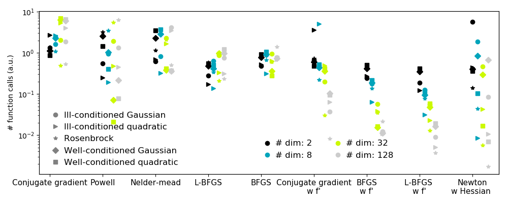
2.7.4.9. Plotting the comparison of optimizers

Plots the results from the comparison of optimizers.

import pickle
import sys

import numpy as np
import matplotlib.pyplot as plt

results = pickle.load(open(
    'helper/compare_optimizers_py%s.pkl' % sys.version_info[0],
    'rb'))
n_methods = len(list(results.values())[0]['Rosenbrock  '])
n_dims = len(results)

symbols = 'o>*Ds'

plt.figure(1, figsize=(10, 4))
plt.clf()

colors = plt.cm.nipy_spectral(np.linspace(0, 1, n_dims))[:, :3]

method_names = list(list(results.values())[0]['Rosenbrock  '].keys())
method_names.sort(key=lambda x: x[::-1], reverse=True)

for n_dim_index, ((n_dim, n_dim_bench), color) in enumerate(
            zip(sorted(results.items()), colors)):
    for (cost_name, cost_bench), symbol in zip(sorted(n_dim_bench.items()),
                    symbols):
        for method_index, method_name, in enumerate(method_names):
            this_bench = cost_bench[method_name]
            bench = np.mean(this_bench)
            plt.semilogy([method_index + .1*n_dim_index, ], [bench, ],
                    marker=symbol, color=color)

# Create a legend for the problem type
for cost_name, symbol in zip(sorted(n_dim_bench.keys()),
            symbols):
    plt.semilogy([-10, ], [0, ], symbol, color='.5',
            label=cost_name)

plt.xticks(np.arange(n_methods), method_names, size=11)
plt.xlim(-.2, n_methods - .5)
plt.legend(loc='best', numpoints=1, handletextpad=0, prop=dict(size=12),
          frameon=False)
plt.ylabel('# function calls (a.u.)')

# Create a second legend for the problem dimensionality
plt.twinx()

for n_dim, color in zip(sorted(results.keys()), colors):
    plt.plot([-10, ], [0, ], 'o', color=color,
            label='# dim: %i' % n_dim)
plt.legend(loc=(.47, .07), numpoints=1, handletextpad=0, prop=dict(size=12),
          frameon=False, ncol=2)
plt.xlim(-.2, n_methods - .5)

plt.xticks(np.arange(n_methods), method_names)
plt.yticks(())

plt.tight_layout()
plt.show()

Total running time of the script: ( 0 minutes 0.612 seconds)