
1.4.5. Some exercises
1.4.5.1. Array manipulations
Form the 2-D array (without typing it in explicitly):
[[1,  6, 11],
 [2,  7, 12],
 [3,  8, 13],
 [4,  9, 14],
 [5, 10, 15]]
and generate a new array containing its 2nd and 4th rows.
Divide each column of the array:
>>> import numpy as np
>>> a = np.arange(25).reshape(5, 5)
elementwise with the array
b = np.array([1., 5, 10, 15, 20]). (Hint:np.newaxis).Harder one: Generate a 10 x 3 array of random numbers (in range [0,1]). For each row, pick the number closest to 0.5.
- Use
absandargsortto find the columnjclosest for each row. - Use fancy indexing to extract the numbers. (Hint:
a[i,j]– the arrayimust contain the row numbers corresponding to stuff inj.)
- Use
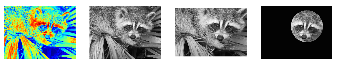
1.4.5.2. Picture manipulation: Framing a Face
Let’s do some manipulations on numpy arrays by starting with an image
of a racoon. scipy provides a 2D array of this image with the
scipy.misc.face function:
>>> from scipy import misc
>>> face = misc.face(gray=True)  # 2D grayscale image
Here are a few images we will be able to obtain with our manipulations: use different colormaps, crop the image, change some parts of the image.
Let’s use the imshow function of matplotlib to display the image.
>>> import matplotlib.pyplot as plt
>>> face = misc.face(gray=True)
>>> plt.imshow(face)
<matplotlib.image.AxesImage object at 0x...>
- The face is displayed in false colors. A colormap must be
specified for it to be displayed in grey.
>>> plt.imshow(face, cmap=plt.cm.gray)
<matplotlib.image.AxesImage object at 0x...>
- Create an array of the image with a narrower centering : for example,
remove 100 pixels from all the borders of the image. To check the result, display this new array with
imshow.>>> crop_face = face[100:-100, 100:-100]
- We will now frame the face with a black locket. For this, we
need to create a mask corresponding to the pixels we want to be black. The center of the face is around (660, 330), so we defined the mask by this condition
(y-300)**2 + (x-660)**2>>> sy, sx = face.shape >>> y, x = np.ogrid[0:sy, 0:sx] # x and y indices of pixels >>> y.shape, x.shape ((768, 1), (1, 1024)) >>> centerx, centery = (660, 300) # center of the image >>> mask = ((y - centery)**2 + (x - centerx)**2) > 230**2 # circle
then we assign the value 0 to the pixels of the image corresponding to the mask. The syntax is extremely simple and intuitive:
>>> face[mask] = 0
>>> plt.imshow(face)
<matplotlib.image.AxesImage object at 0x...>
- Follow-up: copy all instructions of this exercise in a script called
face_locket.pythen execute this script in IPython with%run face_locket.py.Change the circle to an ellipsoid.
1.4.5.3. Data statistics
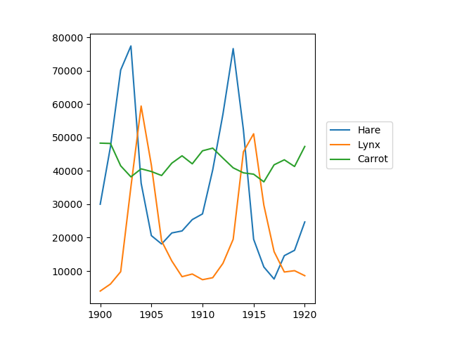
The data in populations.txt
describes the populations of hares and lynxes (and carrots) in
northern Canada during 20 years:
>>> data = np.loadtxt('data/populations.txt')
>>> year, hares, lynxes, carrots = data.T  # trick: columns to variables

>>> import matplotlib.pyplot as plt
>>> plt.axes([0.2, 0.1, 0.5, 0.8])
<matplotlib.axes...Axes object at ...>
>>> plt.plot(year, hares, year, lynxes, year, carrots)
[<matplotlib.lines.Line2D object at ...>, ...]
>>> plt.legend(('Hare', 'Lynx', 'Carrot'), loc=(1.05, 0.5))
<matplotlib.legend.Legend object at ...>
Computes and print, based on the data in populations.txt…
- The mean and std of the populations of each species for the years in the period.
- Which year each species had the largest population.
- Which species has the largest population for each year.
(Hint:
argsort& fancy indexing ofnp.array(['H', 'L', 'C'])) - Which years any of the populations is above 50000.
(Hint: comparisons and
np.any) - The top 2 years for each species when they had the lowest
populations. (Hint:
argsort, fancy indexing) - Compare (plot) the change in hare population (see
help(np.gradient)) and the number of lynxes. Check correlation (seehelp(np.corrcoef)).
… all without for-loops.
Solution: Python source file
1.4.5.4. Crude integral approximations
Write a function f(a, b, c) that returns  . Form
a 24x12x6 array containing its values in parameter ranges
. Form
a 24x12x6 array containing its values in parameter ranges [0,1] x
[0,1] x [0,1].
Approximate the 3-d integral
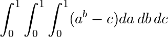
over this volume with the mean. The exact result is: 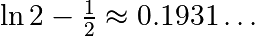 — what is your relative error?
(Hints: use elementwise operations and broadcasting.
You can make np.ogrid give a number of points in given range
with np.ogrid[0:1:20j].)
Reminder Python functions:
def f(a, b, c):
    return some_result
Solution: Python source file
1.4.5.5. Mandelbrot set
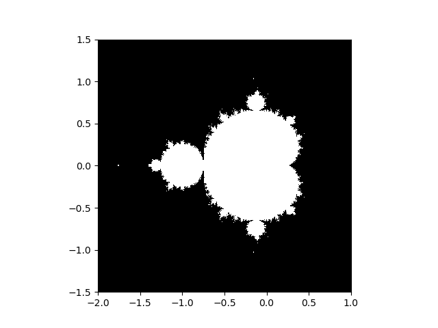
Write a script that computes the Mandelbrot fractal. The Mandelbrot iteration:
N_max = 50
some_threshold = 50

c = x + 1j*y

z = 0
for j in range(N_max):
    z = z**2 + c
Point (x, y) belongs to the Mandelbrot set if  <
<
some_threshold.
Do this computation by:
- Construct a grid of c = x + 1j*y values in range [-2, 1] x [-1.5, 1.5]
- Do the iteration
- Form the 2-d boolean mask indicating which points are in the set
- Save the result to an image with:
>>> import matplotlib.pyplot as plt
>>> plt.imshow(mask.T, extent=[-2, 1, -1.5, 1.5])
<matplotlib.image.AxesImage object at ...>
>>> plt.gray()
>>> plt.savefig('mandelbrot.png')
Solution: Python source file
1.4.5.6. Markov chain

Markov chain transition matrix P, and probability distribution on
the states p:
0 <= P[i,j] <= 1: probability to go from stateito statej- Transition rule:

all(sum(P, axis=1) == 1),p.sum() == 1: normalization
Write a script that works with 5 states, and:
- Constructs a random matrix, and normalizes each row so that it is a transition matrix.
- Starts from a random (normalized) probability distribution
pand takes 50 steps =>p_50 - Computes the stationary distribution: the eigenvector of
P.Twith eigenvalue 1 (numerically: closest to 1) =>p_stationary
Remember to normalize the eigenvector — I didn’t…
- Checks if
p_50andp_stationaryare equal to tolerance 1e-5
Toolbox: np.random.rand, .dot(), np.linalg.eig,
reductions, abs(), argmin, comparisons, all,
np.linalg.norm, etc.
Solution: Python source file