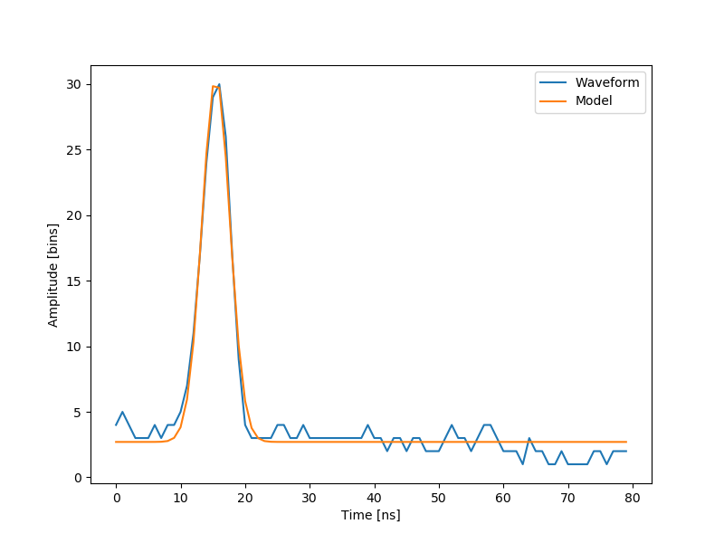
The lidar system, data and fit (1 of 2 datasets)

Generate a chart of the data fitted by Gaussian curve

Out:

[ 2.70363341 27.82020742 15.47924562  3.05636228]

import numpy as np
import matplotlib.pyplot as plt

from scipy.optimize import leastsq


def model(t, coeffs):
    return coeffs[0] + coeffs[1] * np.exp(- ((t-coeffs[2])/coeffs[3])**2)


def residuals(coeffs, y, t):
    return y - model(t, coeffs)


waveform_1 = np.load('waveform_1.npy')
t = np.arange(len(waveform_1))

x0 = np.array([3, 30, 15, 1], dtype=float)
x, flag = leastsq(residuals, x0, args=(waveform_1, t))

print(x)

fig, ax = plt.subplots(figsize=(8, 6))
plt.plot(t, waveform_1, t, model(t, x))
plt.xlabel('Time [ns]')
plt.ylabel('Amplitude [bins]')
plt.legend(['Waveform', 'Model'])
plt.show()

Total running time of the script: ( 0 minutes 0.063 seconds)