3.6.10.15. Example of linear and non-linear models

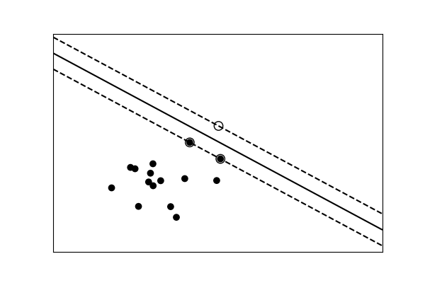
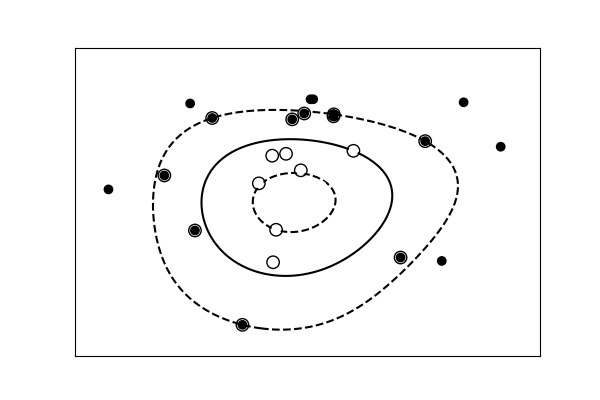
This is an example plot from the tutorial which accompanies an explanation of the support vector machine GUI.

import numpy as np
from matplotlib import pyplot as plt

from sklearn import svm

data that is linearly separable

def linear_model(rseed=42, n_samples=30):
    " Generate data according to a linear model"
    np.random.seed(rseed)

    data = np.random.normal(0, 10, (n_samples, 2))
    data[:n_samples // 2] -= 15
    data[n_samples // 2:] += 15

    labels = np.ones(n_samples)
    labels[:n_samples // 2] = -1

    return data, labels


X, y = linear_model()
clf = svm.SVC(kernel='linear')
clf.fit(X, y)

plt.figure(figsize=(6, 4))
ax = plt.subplot(111, xticks=[], yticks=[])
ax.scatter(X[:, 0], X[:, 1], c=y, cmap=plt.cm.bone)

ax.scatter(clf.support_vectors_[:, 0],
            clf.support_vectors_[:, 1],
            s=80, edgecolors="k", facecolors="none")

delta = 1
y_min, y_max = -50, 50
x_min, x_max = -50, 50
x = np.arange(x_min, x_max + delta, delta)
y = np.arange(y_min, y_max + delta, delta)
X1, X2 = np.meshgrid(x, y)
Z = clf.decision_function(np.c_[X1.ravel(), X2.ravel()])
Z = Z.reshape(X1.shape)

ax.contour(X1, X2, Z, [-1.0, 0.0, 1.0], colors='k',
           linestyles=['dashed', 'solid', 'dashed'])

data with a non-linear separation

def nonlinear_model(rseed=42, n_samples=30):
    radius = 40 * np.random.random(n_samples)
    far_pts = radius > 20
    radius[far_pts] *= 1.2
    radius[~far_pts] *= 1.1

    theta = np.random.random(n_samples) * np.pi * 2

    data = np.empty((n_samples, 2))
    data[:, 0] = radius * np.cos(theta)
    data[:, 1] = radius * np.sin(theta)

    labels = np.ones(n_samples)
    labels[far_pts] = -1

    return data, labels


X, y = nonlinear_model()
clf = svm.SVC(kernel='rbf', gamma=0.001, coef0=0, degree=3)
clf.fit(X, y)

plt.figure(figsize=(6, 4))
ax = plt.subplot(1, 1, 1, xticks=[], yticks=[])
ax.scatter(X[:, 0], X[:, 1], c=y, cmap=plt.cm.bone, zorder=2)

ax.scatter(clf.support_vectors_[:, 0], clf.support_vectors_[:, 1],
           s=80, edgecolors="k", facecolors="none")

delta = 1
y_min, y_max = -50, 50
x_min, x_max = -50, 50
x = np.arange(x_min, x_max + delta, delta)
y = np.arange(y_min, y_max + delta, delta)
X1, X2 = np.meshgrid(x, y)
Z = clf.decision_function(np.c_[X1.ravel(), X2.ravel()])
Z = Z.reshape(X1.shape)

ax.contour(X1, X2, Z, [-1.0, 0.0, 1.0], colors='k',
            linestyles=['dashed', 'solid', 'dashed'], zorder=1)

plt.show()

Total running time of the script: ( 0 minutes 0.047 seconds)