
Note
Click here to download the full example code
3.1.6.8. Air fares before and after 9/11
This is a business-intelligence (BI) like application.
What is interesting here is that we may want to study fares as a function of the year, paired accordingly to the trips, or forgetting the year, only as a function of the trip endpoints.
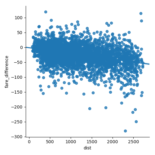
Using statsmodels’ linear models, we find that both with an OLS (ordinary least square) and a robust fit, the intercept and the slope are significantly non-zero: the air fares have decreased between 2000 and 2001, and their dependence on distance travelled has also decreased
# Standard library imports
import urllib
import os
Load the data
import pandas

if not os.path.exists('airfares.txt'):
    # Download the file if it is not present
    urllib.urlretrieve(
        'http://www.stat.ufl.edu/~winner/data/airq4.dat',
                       'airfares.txt')

# As a seperator, ' +' is a regular expression that means 'one of more
# space'
data = pandas.read_csv('airfares.txt', sep=' +', header=0,
                       names=['city1', 'city2', 'pop1', 'pop2',
                              'dist', 'fare_2000', 'nb_passengers_2000',
                              'fare_2001', 'nb_passengers_2001'])

# we log-transform the number of passengers
import numpy as np
data['nb_passengers_2000'] = np.log10(data['nb_passengers_2000'])
data['nb_passengers_2001'] = np.log10(data['nb_passengers_2001'])
Make a dataframe whith the year as an attribute, instead of separate columns
# This involves a small danse in which we separate the dataframes in 2,
# one for year 2000, and one for 2001, before concatenating again.

# Make an index of each flight
data_flat = data.reset_index()

data_2000 = data_flat[['city1', 'city2', 'pop1', 'pop2',
                       'dist', 'fare_2000', 'nb_passengers_2000']]
# Rename the columns
data_2000.columns = ['city1', 'city2', 'pop1', 'pop2', 'dist', 'fare',
                     'nb_passengers']
# Add a column with the year
data_2000['year'] = 2000

data_2001 = data_flat[['city1', 'city2', 'pop1', 'pop2',
                       'dist', 'fare_2001', 'nb_passengers_2001']]
# Rename the columns
data_2001.columns = ['city1', 'city2', 'pop1', 'pop2', 'dist', 'fare',
                     'nb_passengers']
# Add a column with the year
data_2001['year'] = 2001

data_flat = pandas.concat([data_2000, data_2001])
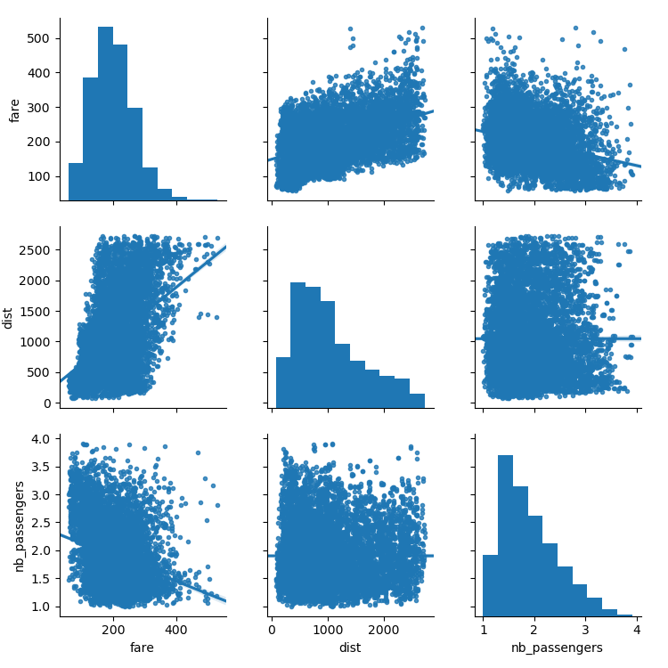
Plot scatter matrices highlighting different aspects
import seaborn
seaborn.pairplot(data_flat, vars=['fare', 'dist', 'nb_passengers'],
kind='reg', markers='.')
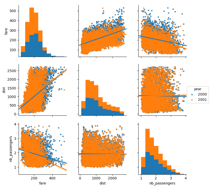
# A second plot, to show the effect of the year (ie the 9/11 effect)
seaborn.pairplot(data_flat, vars=['fare', 'dist', 'nb_passengers'],
kind='reg', hue='year', markers='.')
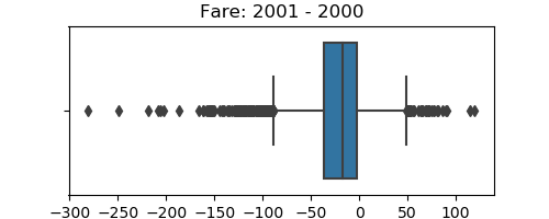
Plot the difference in fare
import matplotlib.pyplot as plt
plt.figure(figsize=(5, 2))
seaborn.boxplot(data.fare_2001 - data.fare_2000)
plt.title('Fare: 2001 - 2000')
plt.subplots_adjust()
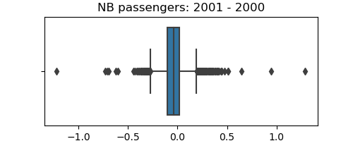
plt.figure(figsize=(5, 2))
seaborn.boxplot(data.nb_passengers_2001 - data.nb_passengers_2000)
plt.title('NB passengers: 2001 - 2000')
plt.subplots_adjust()
Statistical testing: dependence of fare on distance and number of passengers
Out:
OLS Regression Results
==============================================================================
Dep. Variable:                   fare   R-squared:                       0.275
Model:                            OLS   Adj. R-squared:                  0.275
Method:                 Least Squares   F-statistic:                     1585.
Date:                Thu, 18 Aug 2022   Prob (F-statistic):               0.00
Time:                        10:40:20   Log-Likelihood:                -45532.
No. Observations:                8352   AIC:                         9.107e+04
Df Residuals:                    8349   BIC:                         9.109e+04
Df Model:                           2
Covariance Type:            nonrobust
=================================================================================
                    coef    std err          t      P>|t|      [0.025      0.975]
---------------------------------------------------------------------------------
Intercept       211.2428      2.466     85.669      0.000     206.409     216.076
dist              0.0484      0.001     48.149      0.000       0.046       0.050
nb_passengers   -32.8925      1.127    -29.191      0.000     -35.101     -30.684
==============================================================================
Omnibus:                      604.051   Durbin-Watson:                   1.446
Prob(Omnibus):                  0.000   Jarque-Bera (JB):              740.733
Skew:                           0.710   Prob(JB):                    1.42e-161
Kurtosis:                       3.338   Cond. No.                     5.23e+03
==============================================================================

Warnings:
[1] Standard Errors assume that the covariance matrix of the errors is correctly specified.
[2] The condition number is large, 5.23e+03. This might indicate that there are
strong multicollinearity or other numerical problems.
                    Robust linear Model Regression Results
==============================================================================
Dep. Variable:                   fare   No. Observations:                 8352
Model:                            RLM   Df Residuals:                     8349
Method:                          IRLS   Df Model:                            2
Norm:                          HuberT
Scale Est.:                       mad
Cov Type:                          H1
Date:                Thu, 18 Aug 2022
Time:                        10:40:20
No. Iterations:                    12
=================================================================================
                    coef    std err          z      P>|z|      [0.025      0.975]
---------------------------------------------------------------------------------
Intercept       215.0848      2.448     87.856      0.000     210.287     219.883
dist              0.0460      0.001     46.166      0.000       0.044       0.048
nb_passengers   -35.2686      1.119    -31.526      0.000     -37.461     -33.076
=================================================================================

If the model instance has been used for another fit with different fit
parameters, then the fit options might not be the correct ones anymore .
Statistical testing: regression of fare on distance: 2001/2000 difference
result = sm.ols(formula='fare_2001 - fare_2000 ~ 1 + dist', data=data).fit()
print(result.summary())

# Plot the corresponding regression
data['fare_difference'] = data['fare_2001'] - data['fare_2000']
seaborn.lmplot(x='dist', y='fare_difference', data=data)

plt.show()
Out:
OLS Regression Results
==============================================================================
Dep. Variable:              fare_2001   R-squared:                       0.159
Model:                            OLS   Adj. R-squared:                  0.159
Method:                 Least Squares   F-statistic:                     791.7
Date:                Thu, 18 Aug 2022   Prob (F-statistic):          1.20e-159
Time:                        10:40:20   Log-Likelihood:                -22640.
No. Observations:                4176   AIC:                         4.528e+04
Df Residuals:                    4174   BIC:                         4.530e+04
Df Model:                           1
Covariance Type:            nonrobust
==============================================================================
                 coef    std err          t      P>|t|      [0.025      0.975]
------------------------------------------------------------------------------
Intercept    148.0279      1.673     88.480      0.000     144.748     151.308
dist           0.0388      0.001     28.136      0.000       0.036       0.041
==============================================================================
Omnibus:                      136.558   Durbin-Watson:                   1.544
Prob(Omnibus):                  0.000   Jarque-Bera (JB):              149.624
Skew:                           0.462   Prob(JB):                     3.23e-33
Kurtosis:                       2.920   Cond. No.                     2.40e+03
==============================================================================

Warnings:
[1] Standard Errors assume that the covariance matrix of the errors is correctly specified.
[2] The condition number is large, 2.4e+03. This might indicate that there are
strong multicollinearity or other numerical problems.
Total running time of the script: ( 0 minutes 8.753 seconds)