
2.6. Image manipulation and processing using Numpy and Scipy
Authors: Emmanuelle Gouillart, Gaël Varoquaux
This section addresses basic image manipulation and processing using the
core scientific modules NumPy and SciPy. Some of the operations covered
by this tutorial may be useful for other kinds of multidimensional array
processing than image processing. In particular, the submodule
scipy.ndimage provides functions operating on n-dimensional NumPy
arrays.
See also
For more advanced image processing and image-specific routines, see the
tutorial Scikit-image: image processing, dedicated to the skimage module.
Image = 2-D numerical array
(or 3-D: CT, MRI, 2D + time; 4-D, …)
Here, image == Numpy array np.array
Tools used in this tutorial:
numpy: basic array manipulationscipy:scipy.ndimagesubmodule dedicated to image processing (n-dimensional images). See the documentation:>>> from scipy import ndimage
Common tasks in image processing:
- Input/Output, displaying images
- Basic manipulations: cropping, flipping, rotating, …
- Image filtering: denoising, sharpening
- Image segmentation: labeling pixels corresponding to different objects
- Classification
- Feature extraction
- Registration
- …
Chapters contents
2.6.1. Opening and writing to image files
Writing an array to a file:
from scipy import misc
import imageio
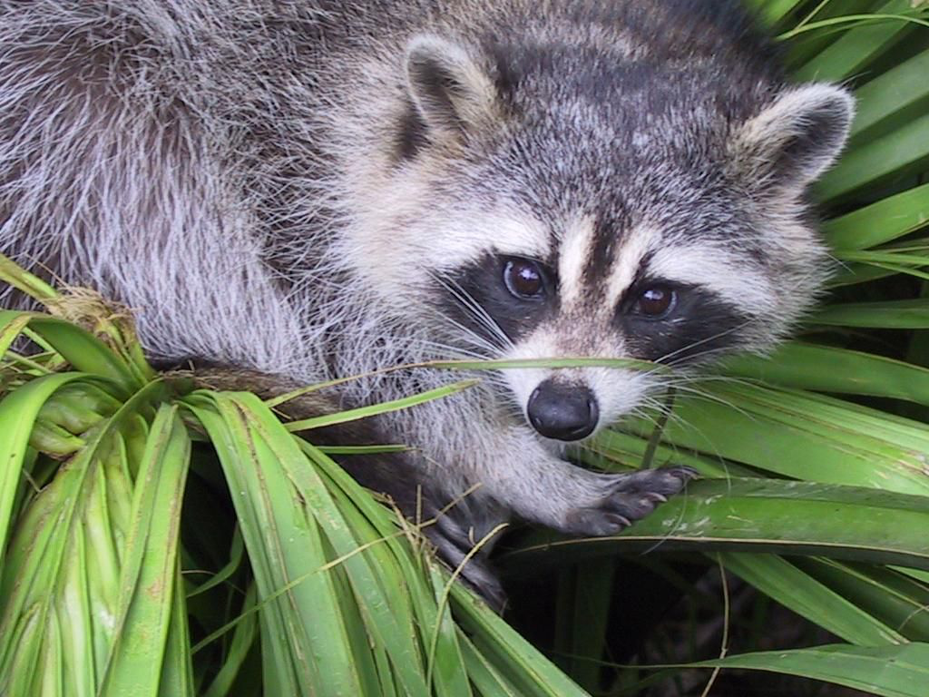
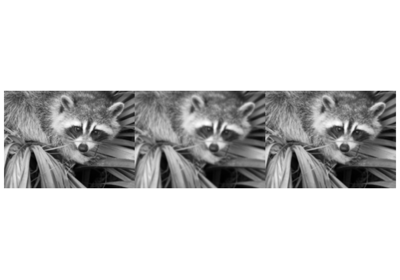
f = misc.face()
imageio.imsave('face.png', f) # uses the Image module (PIL)
import matplotlib.pyplot as plt
plt.imshow(f)
plt.show()
Creating a numpy array from an image file:
>>> from scipy import misc
>>> import imageio
>>> face = misc.face()
>>> imageio.imsave('face.png', face) # First we need to create the PNG file

>>> face = imageio.imread('face.png')
>>> type(face)
<class 'imageio.core.util.Array'>
>>> face.shape, face.dtype
((768, 1024, 3), dtype('uint8'))
dtype is uint8 for 8-bit images (0-255)
Opening raw files (camera, 3-D images)
>>> face.tofile('face.raw') # Create raw file
>>> face_from_raw = np.fromfile('face.raw', dtype=np.uint8)
>>> face_from_raw.shape
(2359296,)
>>> face_from_raw.shape = (768, 1024, 3)
Need to know the shape and dtype of the image (how to separate data bytes).
For large data, use np.memmap for memory mapping:
>>> face_memmap = np.memmap('face.raw', dtype=np.uint8, shape=(768, 1024, 3))
(data are read from the file, and not loaded into memory)
Working on a list of image files
>>> for i in range(10):
...     im = np.random.randint(0, 256, 10000).reshape((100, 100))
...     imageio.imsave('random_%02d.png' % i, im)
>>> from glob import glob
>>> filelist = glob('random*.png')
>>> filelist.sort()
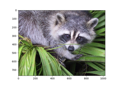
2.6.2. Displaying images
Use matplotlib and imshow to display an image inside a
matplotlib figure:
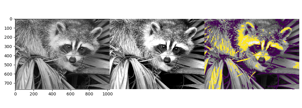
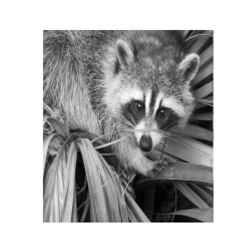
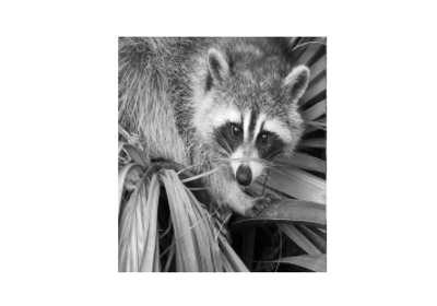
>>> f = misc.face(gray=True)  # retrieve a grayscale image
>>> import matplotlib.pyplot as plt
>>> plt.imshow(f, cmap=plt.cm.gray)
<matplotlib.image.AxesImage object at 0x...>
Increase contrast by setting min and max values:
>>> plt.imshow(f, cmap=plt.cm.gray, vmin=30, vmax=200)
<matplotlib.image.AxesImage object at 0x...>
>>> # Remove axes and ticks
>>> plt.axis('off')
(-0.5, 1023.5, 767.5, -0.5)
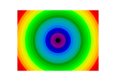
Draw contour lines:
>>> plt.contour(f, [50, 200])
<matplotlib.contour.QuadContourSet ...>
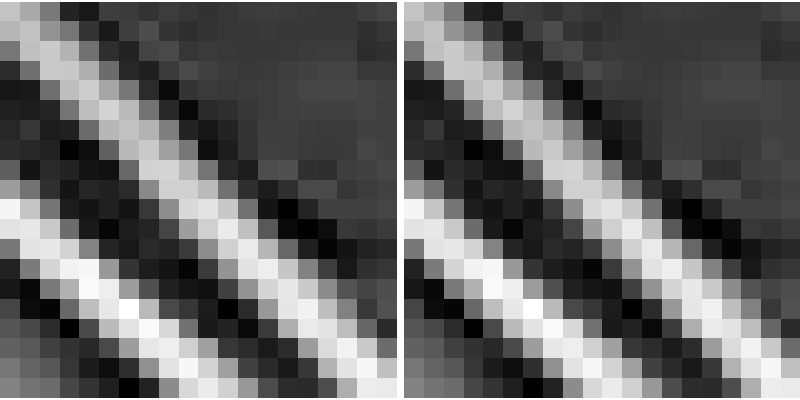
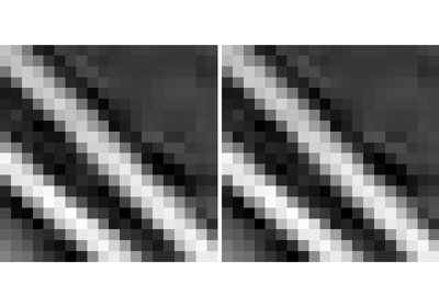
For smooth intensity variations, use interpolation='bilinear'. For fine inspection of intensity variations, use
interpolation='nearest':
>>> plt.imshow(f[320:340, 510:530], cmap=plt.cm.gray, interpolation='bilinear')
<matplotlib.image.AxesImage object at 0x...>
>>> plt.imshow(f[320:340, 510:530], cmap=plt.cm.gray, interpolation='nearest')
<matplotlib.image.AxesImage object at 0x...>
See also
More interpolation methods are in Matplotlib’s examples.
2.6.3. Basic manipulations
Images are arrays: use the whole numpy machinery.
>>> face = misc.face(gray=True)
>>> face[0, 40]
127
>>> # Slicing
>>> face[10:13, 20:23]
array([[141, 153, 145],
[133, 134, 125],
[ 96, 92, 94]], dtype=uint8)
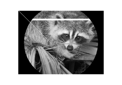
>>> face[100:120] = 255
>>>
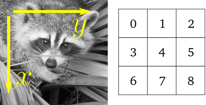
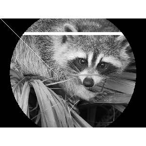
>>> lx, ly = face.shape
>>> X, Y = np.ogrid[0:lx, 0:ly]
>>> mask = (X - lx / 2) ** 2 + (Y - ly / 2) ** 2 > lx * ly / 4
>>> # Masks
>>> face[mask] = 0
>>> # Fancy indexing
>>> face[range(400), range(400)] = 255
2.6.3.1. Statistical information
>>> face = misc.face(gray=True)
>>> face.mean()
113.48026784261067
>>> face.max(), face.min()
(250, 0)
np.histogram
Exercise
- Open as an array the
scikit-imagelogo (http://scikit-image.org/_static/img/logo.png), or an image that you have on your computer. - Crop a meaningful part of the image, for example the python circle in the logo.
- Display the image array using
matplotlib. Change the interpolation method and zoom to see the difference. - Transform your image to greyscale
- Increase the contrast of the image by changing its minimum and
maximum values. Optional: use
scipy.stats.scoreatpercentile(read the docstring!) to saturate 5% of the darkest pixels and 5% of the lightest pixels. - Save the array to two different file formats (png, jpg, tiff)
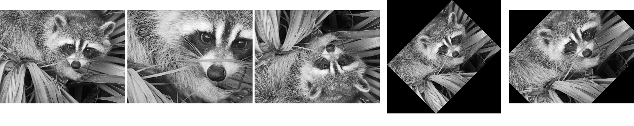
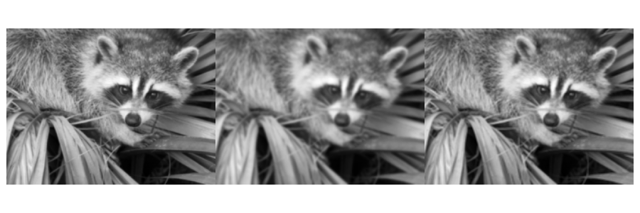
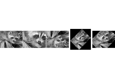
2.6.3.2. Geometrical transformations
>>> face = misc.face(gray=True)
>>> lx, ly = face.shape
>>> # Cropping
>>> crop_face = face[lx // 4: - lx // 4, ly // 4: - ly // 4]
>>> # up <-> down flip
>>> flip_ud_face = np.flipud(face)
>>> # rotation
>>> rotate_face = ndimage.rotate(face, 45)
>>> rotate_face_noreshape = ndimage.rotate(face, 45, reshape=False)
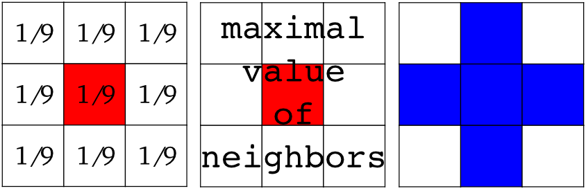
2.6.4. Image filtering
Local filters: replace the value of pixels by a function of the values of neighboring pixels.
Neighbourhood: square (choose size), disk, or more complicated structuring element.
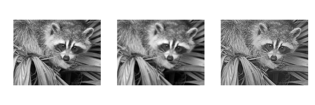
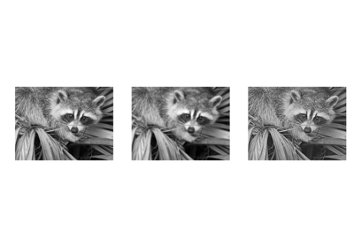
2.6.4.1. Blurring/smoothing
Gaussian filter from scipy.ndimage:
>>> from scipy import misc
>>> face = misc.face(gray=True)
>>> blurred_face = ndimage.gaussian_filter(face, sigma=3)
>>> very_blurred = ndimage.gaussian_filter(face, sigma=5)
Uniform filter
>>> local_mean = ndimage.uniform_filter(face, size=11)
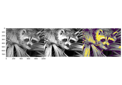
2.6.4.2. Sharpening
Sharpen a blurred image:
>>> from scipy import misc
>>> face = misc.face(gray=True).astype(float)
>>> blurred_f = ndimage.gaussian_filter(face, 3)
increase the weight of edges by adding an approximation of the Laplacian:
>>> filter_blurred_f = ndimage.gaussian_filter(blurred_f, 1)
>>> alpha = 30
>>> sharpened = blurred_f + alpha * (blurred_f - filter_blurred_f)
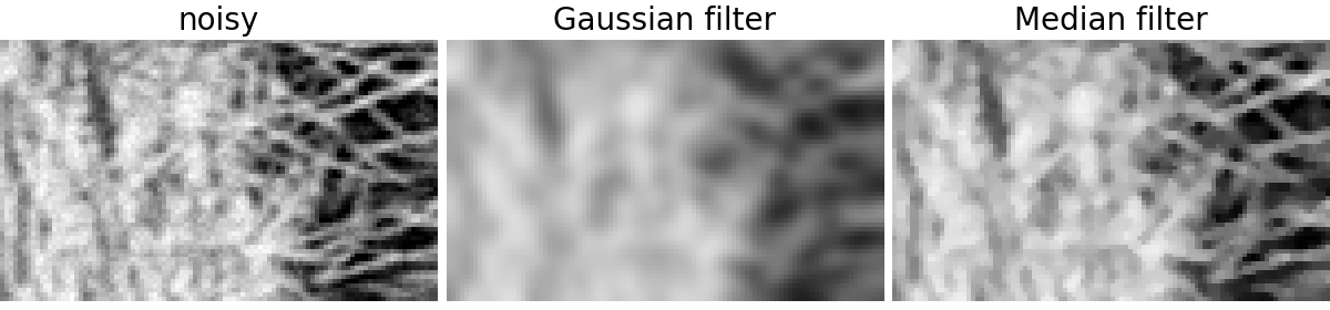
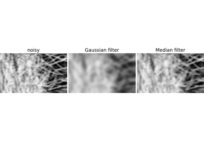
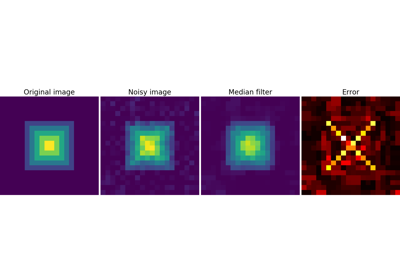
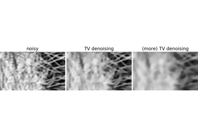
2.6.4.3. Denoising
Noisy face:
>>> from scipy import misc
>>> f = misc.face(gray=True)
>>> f = f[230:290, 220:320]
>>> noisy = f + 0.4 * f.std() * np.random.random(f.shape)
A Gaussian filter smoothes the noise out… and the edges as well:
>>> gauss_denoised = ndimage.gaussian_filter(noisy, 2)
Most local linear isotropic filters blur the image (ndimage.uniform_filter)
A median filter preserves better the edges:
>>> med_denoised = ndimage.median_filter(noisy, 3)
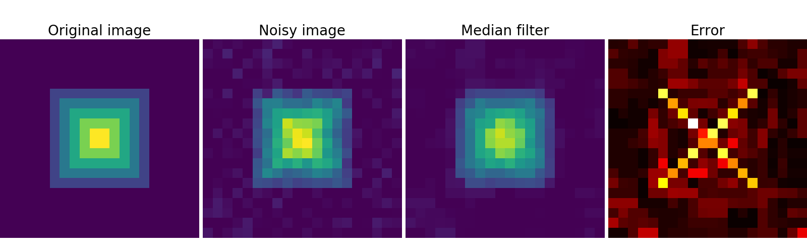
Median filter: better result for straight boundaries (low curvature):
>>> im = np.zeros((20, 20))
>>> im[5:-5, 5:-5] = 1
>>> im = ndimage.distance_transform_bf(im)
>>> im_noise = im + 0.2 * np.random.randn(*im.shape)
>>> im_med = ndimage.median_filter(im_noise, 3)
Other rank filter: ndimage.maximum_filter,
ndimage.percentile_filter
Other local non-linear filters: Wiener (scipy.signal.wiener), etc.
Non-local filters
Exercise: denoising
- Create a binary image (of 0s and 1s) with several objects (circles, ellipses, squares, or random shapes).
- Add some noise (e.g., 20% of noise)
- Try two different denoising methods for denoising the image: gaussian filtering and median filtering.
- Compare the histograms of the two different denoised images. Which one is the closest to the histogram of the original (noise-free) image?
See also
More denoising filters are available in skimage.denoising,
see the Scikit-image: image processing tutorial.
2.6.4.4. Mathematical morphology
See wikipedia for a definition of mathematical morphology.
Probe an image with a simple shape (a structuring element), and modify this image according to how the shape locally fits or misses the image.
Structuring element:
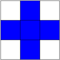
>>> el = ndimage.generate_binary_structure(2, 1)
>>> el
array([[False,  True, False],
       [ True,  True,  True],
       [False,  True, False]])
>>> el.astype(np.int)
array([[0, 1, 0],
       [1, 1, 1],
       [0, 1, 0]])
Erosion = minimum filter. Replace the value of a pixel by the minimal value covered by the structuring element.:
>>> a = np.zeros((7,7), dtype=np.int)
>>> a[1:6, 2:5] = 1
>>> a
array([[0, 0, 0, 0, 0, 0, 0],
       [0, 0, 1, 1, 1, 0, 0],
       [0, 0, 1, 1, 1, 0, 0],
       [0, 0, 1, 1, 1, 0, 0],
       [0, 0, 1, 1, 1, 0, 0],
       [0, 0, 1, 1, 1, 0, 0],
       [0, 0, 0, 0, 0, 0, 0]])
>>> ndimage.binary_erosion(a).astype(a.dtype)
array([[0, 0, 0, 0, 0, 0, 0],
       [0, 0, 0, 0, 0, 0, 0],
       [0, 0, 0, 1, 0, 0, 0],
       [0, 0, 0, 1, 0, 0, 0],
       [0, 0, 0, 1, 0, 0, 0],
       [0, 0, 0, 0, 0, 0, 0],
       [0, 0, 0, 0, 0, 0, 0]])
>>> #Erosion removes objects smaller than the structure
>>> ndimage.binary_erosion(a, structure=np.ones((5,5))).astype(a.dtype)
array([[0, 0, 0, 0, 0, 0, 0],
       [0, 0, 0, 0, 0, 0, 0],
       [0, 0, 0, 0, 0, 0, 0],
       [0, 0, 0, 0, 0, 0, 0],
       [0, 0, 0, 0, 0, 0, 0],
       [0, 0, 0, 0, 0, 0, 0],
       [0, 0, 0, 0, 0, 0, 0]])
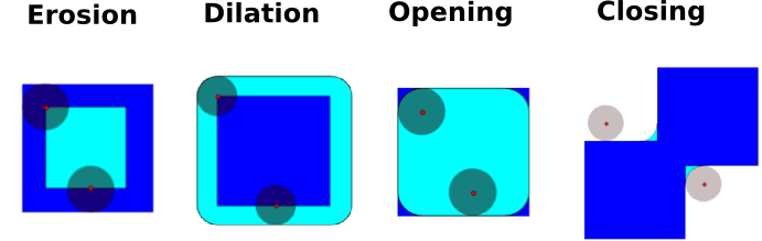
Dilation: maximum filter:
>>> a = np.zeros((5, 5))
>>> a[2, 2] = 1
>>> a
array([[0.,  0.,  0.,  0.,  0.],
       [0.,  0.,  0.,  0.,  0.],
       [0.,  0.,  1.,  0.,  0.],
       [0.,  0.,  0.,  0.,  0.],
       [0.,  0.,  0.,  0.,  0.]])
>>> ndimage.binary_dilation(a).astype(a.dtype)
array([[0.,  0.,  0.,  0.,  0.],
       [0.,  0.,  1.,  0.,  0.],
       [0.,  1.,  1.,  1.,  0.],
       [0.,  0.,  1.,  0.,  0.],
       [0.,  0.,  0.,  0.,  0.]])
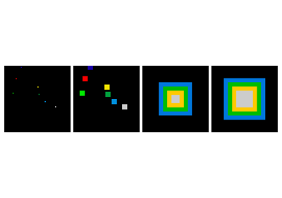
Also works for grey-valued images:
>>> np.random.seed(2)
>>> im = np.zeros((64, 64))
>>> x, y = (63*np.random.random((2, 8))).astype(np.int)
>>> im[x, y] = np.arange(8)

>>> bigger_points = ndimage.grey_dilation(im, size=(5, 5), structure=np.ones((5, 5)))

>>> square = np.zeros((16, 16))
>>> square[4:-4, 4:-4] = 1
>>> dist = ndimage.distance_transform_bf(square)
>>> dilate_dist = ndimage.grey_dilation(dist, size=(3, 3), \
...         structure=np.ones((3, 3)))

Opening: erosion + dilation:
>>> a = np.zeros((5,5), dtype=np.int)
>>> a[1:4, 1:4] = 1; a[4, 4] = 1
>>> a
array([[0, 0, 0, 0, 0],
       [0, 1, 1, 1, 0],
       [0, 1, 1, 1, 0],
       [0, 1, 1, 1, 0],
       [0, 0, 0, 0, 1]])
>>> # Opening removes small objects
>>> ndimage.binary_opening(a, structure=np.ones((3,3))).astype(np.int)
array([[0, 0, 0, 0, 0],
       [0, 1, 1, 1, 0],
       [0, 1, 1, 1, 0],
       [0, 1, 1, 1, 0],
       [0, 0, 0, 0, 0]])
>>> # Opening can also smooth corners
>>> ndimage.binary_opening(a).astype(np.int)
array([[0, 0, 0, 0, 0],
       [0, 0, 1, 0, 0],
       [0, 1, 1, 1, 0],
       [0, 0, 1, 0, 0],
       [0, 0, 0, 0, 0]])
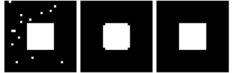
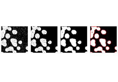
Application: remove noise:
>>> square = np.zeros((32, 32))
>>> square[10:-10, 10:-10] = 1
>>> np.random.seed(2)
>>> x, y = (32*np.random.random((2, 20))).astype(np.int)
>>> square[x, y] = 1

>>> open_square = ndimage.binary_opening(square)

>>> eroded_square = ndimage.binary_erosion(square)
>>> reconstruction = ndimage.binary_propagation(eroded_square, mask=square)
Closing: dilation + erosion
Many other mathematical morphology operations: hit and miss transform, tophat, etc.
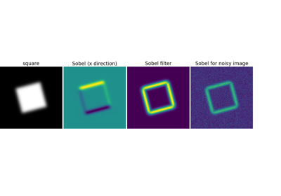
2.6.5. Feature extraction
2.6.5.1. Edge detection
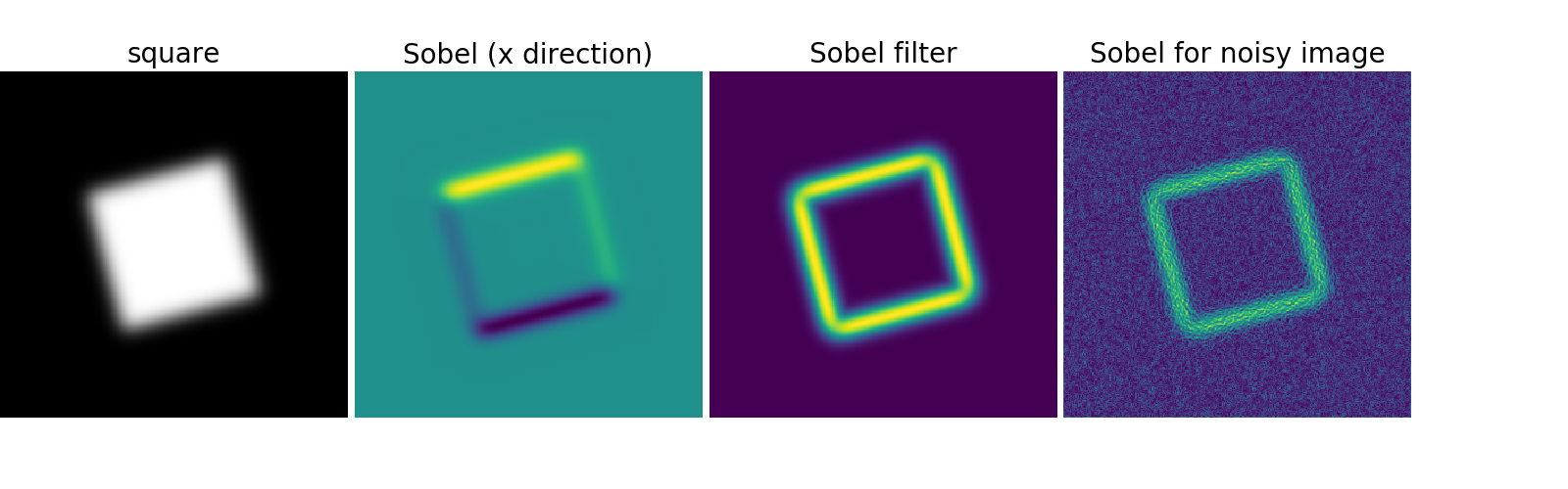
Synthetic data:
>>> im = np.zeros((256, 256))
>>> im[64:-64, 64:-64] = 1
>>>
>>> im = ndimage.rotate(im, 15, mode='constant')
>>> im = ndimage.gaussian_filter(im, 8)
Use a gradient operator (Sobel) to find high intensity variations:
>>> sx = ndimage.sobel(im, axis=0, mode='constant')
>>> sy = ndimage.sobel(im, axis=1, mode='constant')
>>> sob = np.hypot(sx, sy)
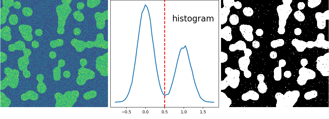
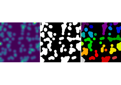
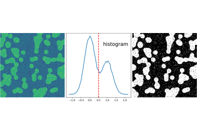
2.6.5.2. Segmentation
- Histogram-based segmentation (no spatial information)
>>> n = 10
>>> l = 256
>>> im = np.zeros((l, l))
>>> np.random.seed(1)
>>> points = l*np.random.random((2, n**2))
>>> im[(points[0]).astype(np.int), (points[1]).astype(np.int)] = 1
>>> im = ndimage.gaussian_filter(im, sigma=l/(4.*n))
>>> mask = (im > im.mean()).astype(np.float)
>>> mask += 0.1 * im
>>> img = mask + 0.2*np.random.randn(*mask.shape)
>>> hist, bin_edges = np.histogram(img, bins=60)
>>> bin_centers = 0.5*(bin_edges[:-1] + bin_edges[1:])
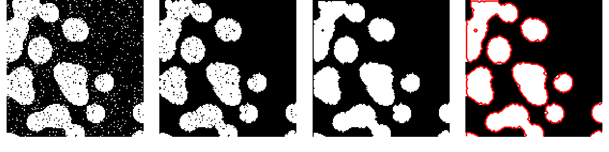
>>> binary_img = img > 0.5
Use mathematical morphology to clean up the result:
>>> # Remove small white regions
>>> open_img = ndimage.binary_opening(binary_img)
>>> # Remove small black hole
>>> close_img = ndimage.binary_closing(open_img)
Exercise
Check that reconstruction operations (erosion + propagation) produce a better result than opening/closing:
>>> eroded_img = ndimage.binary_erosion(binary_img)
>>> reconstruct_img = ndimage.binary_propagation(eroded_img, mask=binary_img)
>>> tmp = np.logical_not(reconstruct_img)
>>> eroded_tmp = ndimage.binary_erosion(tmp)
>>> reconstruct_final = np.logical_not(ndimage.binary_propagation(eroded_tmp, mask=tmp))
>>> np.abs(mask - close_img).mean()
0.00727836...
>>> np.abs(mask - reconstruct_final).mean()
0.00059502...
Exercise
Check how a first denoising step (e.g. with a median filter) modifies the histogram, and check that the resulting histogram-based segmentation is more accurate.
See also
More advanced segmentation algorithms are found in the
scikit-image: see Scikit-image: image processing.
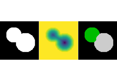
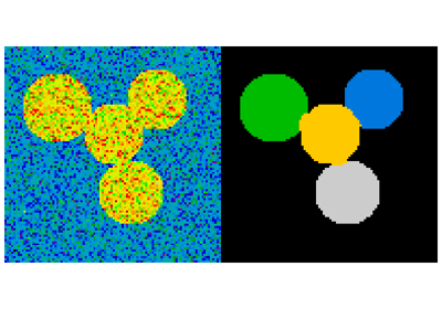
See also
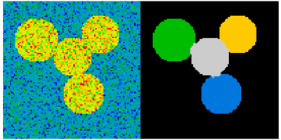
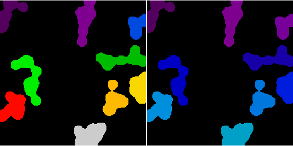
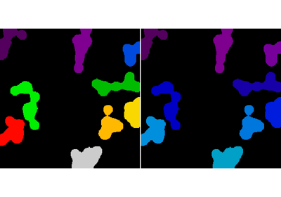
Other Scientific Packages provide algorithms that can be useful for
image processing. In this example, we use the spectral clustering
function of the scikit-learn in order to segment glued objects.
>>> from sklearn.feature_extraction import image
>>> from sklearn.cluster import spectral_clustering

>>> l = 100
>>> x, y = np.indices((l, l))

>>> center1 = (28, 24)
>>> center2 = (40, 50)
>>> center3 = (67, 58)
>>> center4 = (24, 70)
>>> radius1, radius2, radius3, radius4 = 16, 14, 15, 14

>>> circle1 = (x - center1[0])**2 + (y - center1[1])**2 < radius1**2
>>> circle2 = (x - center2[0])**2 + (y - center2[1])**2 < radius2**2
>>> circle3 = (x - center3[0])**2 + (y - center3[1])**2 < radius3**2
>>> circle4 = (x - center4[0])**2 + (y - center4[1])**2 < radius4**2

>>> # 4 circles
>>> img = circle1 + circle2 + circle3 + circle4
>>> mask = img.astype(bool)
>>> img = img.astype(float)

>>> img += 1 + 0.2*np.random.randn(*img.shape)
>>> # Convert the image into a graph with the value of the gradient on
>>> # the edges.
>>> graph = image.img_to_graph(img, mask=mask)

>>> # Take a decreasing function of the gradient: we take it weakly
>>> # dependant from the gradient the segmentation is close to a voronoi
>>> graph.data = np.exp(-graph.data/graph.data.std())

>>> labels = spectral_clustering(graph, n_clusters=4, eigen_solver='arpack')
>>> label_im = -np.ones(mask.shape)
>>> label_im[mask] = labels
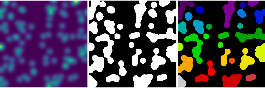
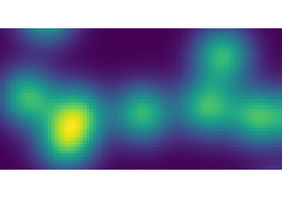
2.6.6. Measuring objects properties: ndimage.measurements
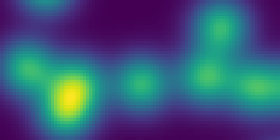
Synthetic data:
>>> n = 10
>>> l = 256
>>> im = np.zeros((l, l))
>>> points = l*np.random.random((2, n**2))
>>> im[(points[0]).astype(np.int), (points[1]).astype(np.int)] = 1
>>> im = ndimage.gaussian_filter(im, sigma=l/(4.*n))
>>> mask = im > im.mean()
- Analysis of connected components
Label connected components: ndimage.label:
>>> label_im, nb_labels = ndimage.label(mask)
>>> nb_labels # how many regions?
29
>>> plt.imshow(label_im)
<matplotlib.image.AxesImage object at 0x...>
Compute size, mean_value, etc. of each region:
>>> sizes = ndimage.sum(mask, label_im, range(nb_labels + 1))
>>> mean_vals = ndimage.sum(im, label_im, range(1, nb_labels + 1))
Clean up small connect components:
>>> mask_size = sizes < 1000
>>> remove_pixel = mask_size[label_im]
>>> remove_pixel.shape
(256, 256)
>>> label_im[remove_pixel] = 0
>>> plt.imshow(label_im)
<matplotlib.image.AxesImage object at 0x...>
Now reassign labels with np.searchsorted:
>>> labels = np.unique(label_im)
>>> label_im = np.searchsorted(labels, label_im)
Find region of interest enclosing object:
>>> slice_x, slice_y = ndimage.find_objects(label_im==4)[0]
>>> roi = im[slice_x, slice_y]
>>> plt.imshow(roi)
<matplotlib.image.AxesImage object at 0x...>
Other spatial measures: ndimage.center_of_mass,
ndimage.maximum_position, etc.
Can be used outside the limited scope of segmentation applications.
Example: block mean:
>>> from scipy import misc
>>> f = misc.face(gray=True)
>>> sx, sy = f.shape
>>> X, Y = np.ogrid[0:sx, 0:sy]
>>> regions = (sy//6) * (X//4) + (Y//6)  # note that we use broadcasting
>>> block_mean = ndimage.mean(f, labels=regions, index=np.arange(1,
...     regions.max() +1))
>>> block_mean.shape = (sx // 4, sy // 6)
When regions are regular blocks, it is more efficient to use stride tricks (Example: fake dimensions with strides).
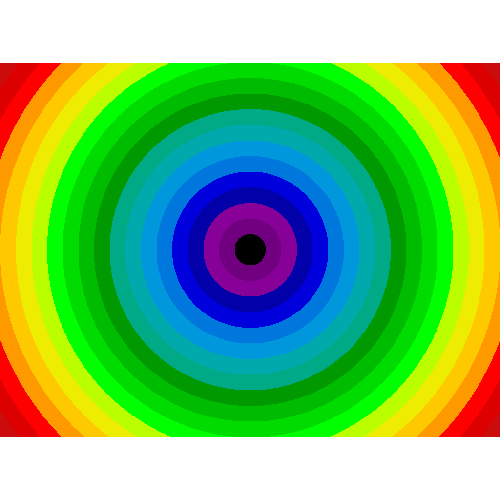
Non-regularly-spaced blocks: radial mean:
>>> sx, sy = f.shape
>>> X, Y = np.ogrid[0:sx, 0:sy]
>>> r = np.hypot(X - sx/2, Y - sy/2)
>>> rbin = (20* r/r.max()).astype(np.int)
>>> radial_mean = ndimage.mean(f, labels=rbin, index=np.arange(1, rbin.max() +1))
- Other measures
Correlation function, Fourier/wavelet spectrum, etc.
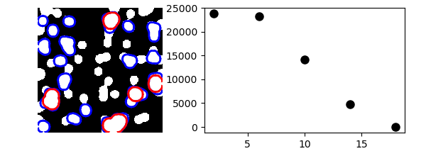
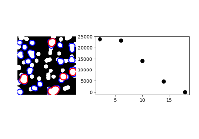
One example with mathematical morphology: granulometry
>>> def disk_structure(n):
...     struct = np.zeros((2 * n + 1, 2 * n + 1))
...     x, y = np.indices((2 * n + 1, 2 * n + 1))
...     mask = (x - n)**2 + (y - n)**2 <= n**2
...     struct[mask] = 1
...     return struct.astype(np.bool)
...
>>>
>>> def granulometry(data, sizes=None):
...     s = max(data.shape)
...     if sizes is None:
...         sizes = range(1, s/2, 2)
...     granulo = [ndimage.binary_opening(data, \
...         structure=disk_structure(n)).sum() for n in sizes]
...     return granulo
...
>>>
>>> np.random.seed(1)
>>> n = 10
>>> l = 256
>>> im = np.zeros((l, l))
>>> points = l*np.random.random((2, n**2))
>>> im[(points[0]).astype(np.int), (points[1]).astype(np.int)] = 1
>>> im = ndimage.gaussian_filter(im, sigma=l/(4.*n))
>>>
>>> mask = im > im.mean()
>>>
>>> granulo = granulometry(mask, sizes=np.arange(2, 19, 4))
2.6.8. Examples for the image processing chapter


Gallery generated by Sphinx-Gallery
See also
More on image-processing:
- The chapter on Scikit-image
- Other, more powerful and complete modules: OpenCV (Python bindings), CellProfiler, ITK with Python bindings