2.7. Mathematical optimization: finding minima of functions¶

Authors: Gaël Varoquaux

Mathematical optimization deals with the problem of finding numerically minimums (or maximums or zeros) of a function. In this context, the function is called cost function, or objective function, or energy.

Here, we are interested in using scipy.optimize for black-box optimization: we do not rely on the mathematical expression of the function that we are optimizing. Note that this expression can often be used for more efficient, non black-box, optimization.

Prerequisites

2.7.1. Knowing your problem ¶

Not all optimization problems are equal. Knowing your problem enables you to choose the right tool.

Dimensionality of the problem

The scale of an optimization problem is pretty much set by the dimensionality of the problem, i.e. the number of scalar variables on which the search is performed.

2.7.1.1. Convex versus non-convex optimization ¶

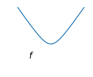
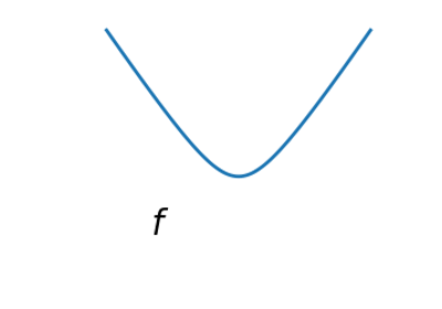
A convex function:

f is above all its tangents.
equivalently, for two point A, B, f(C) lies below the segment [f(A), f(B])], if A < C < B

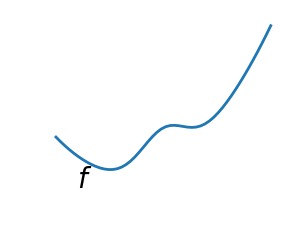
A non-convex function

Optimizing convex functions is easy. Optimizing non-convex functions can be very hard.

Note

It can be proven that for a convex function a local minimum is also a global minimum. Then, in some sense, the minimum is unique.

2.7.1.2. Smooth and non-smooth problems ¶

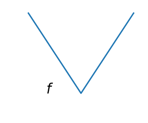A smooth function:

The gradient is defined everywhere, and is a continuous function

A non-smooth function

Optimizing smooth functions is easier (true in the context of black-box optimization, otherwise Linear Programming is an example of methods which deal very efficiently with piece-wise linear functions).

2.7.1.3. Noisy versus exact cost functions ¶

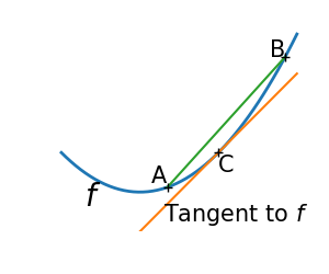
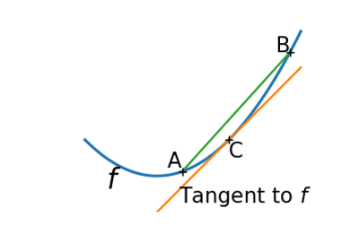
Noisy (blue) and non-noisy (green) functions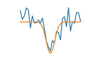

Noisy gradients

Many optimization methods rely on gradients of the objective function. If the gradient function is not given, they are computed numerically, which induces errors. In such situation, even if the objective function is not noisy, a gradient-based optimization may be a noisy optimization.

2.7.1.4. Constraints ¶

Optimizations under constraints

Here:

$-1 < x_1 < 1$

$-1 < x_2 < 1$

2.7.2. A review of the different optimizers ¶

2.7.2.1. Getting started: 1D optimization ¶

Let’s get started by finding the minimum of the scalar function $f(x)=\exp[(x-0.7)^2]$ . scipy.optimize.minimize_scalar() uses Brent’s method to find the minimum of a function:

>>> fromscipyimportoptimize
>>> deff(x):
... return-np.exp(-(x-0.7)**2)
>>> result=optimize.minimize_scalar(f)
>>> result.success# check if solver was successful
True
>>> x_min=result.x
>>> x_min
0.699999999...
>>> x_min-0.7
-2.16...e-10

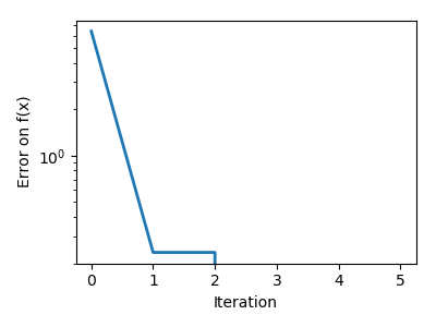
Brent’s method on a quadratic function: it converges in 3 iterations, as the quadratic approximation is then exact.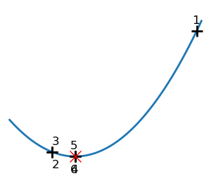
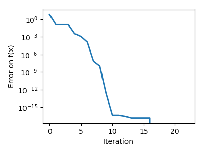
Brent’s method on a non-convex function: note that the fact that the optimizer avoided the local minimum is a matter of luck.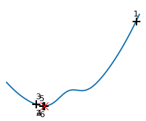

Note

You can use different solvers using the parameter method.

Note

scipy.optimize.minimize_scalar() can also be used for optimization constrained to an interval using the parameter bounds.

2.7.2.2. Gradient based methods ¶

Some intuitions about gradient descent¶

Here we focus on intuitions, not code. Code will follow.

Gradient descent basically consists in taking small steps in the direction of the gradient, that is the direction of the steepest descent.

**Fixed step gradient descent**¶
A well-conditioned quadratic function.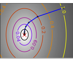
An ill-conditioned quadratic function. The core problem of gradient-methods on ill-conditioned problems is that the gradient tends not to point in the direction of the minimum.

We can see that very anisotropic (ill-conditioned) functions are harder to optimize.

Take home message: conditioning number and preconditioning

If you know natural scaling for your variables, prescale them so that they behave similarly. This is related to preconditioning.

Also, it clearly can be advantageous to take bigger steps. This is done in gradient descent code using a line search.

**Adaptive step gradient descent**¶
A well-conditioned quadratic function.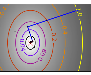
An ill-conditioned quadratic function.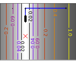
An ill-conditioned non-quadratic function.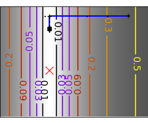
An ill-conditioned very non-quadratic function.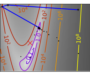

The more a function looks like a quadratic function (elliptic iso-curves), the easier it is to optimize.

Conjugate gradient descent¶

The gradient descent algorithms above are toys not to be used on real problems.

As can be seen from the above experiments, one of the problems of the simple gradient descent algorithms, is that it tends to oscillate across a valley, each time following the direction of the gradient, that makes it cross the valley. The conjugate gradient solves this problem by adding a friction term: each step depends on the two last values of the gradient and sharp turns are reduced.

**Conjugate gradient descent**¶
An ill-conditioned non-quadratic function.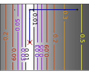
An ill-conditioned very non-quadratic function.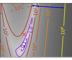

scipy provides scipy.optimize.minimize() to find the minimum of scalar functions of one or more variables. The simple conjugate gradient method can be used by setting the parameter method to CG

>>> deff(x):# The rosenbrock function
... return.5*(1-x[0])**2+(x[1]-x[0]**2)**2
>>> optimize.minimize(f,[2,-1],method="CG")
     fun: 1.6...e-11
     jac: array([-6.15...e-06,   2.53...e-07])
 message: ...'Optimization terminated successfully.'
    nfev: 108
     nit: 13
    njev: 27
  status: 0
 success: True
       x: array([0.99999...,  0.99998...])

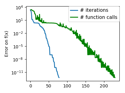
Gradient methods need the Jacobian (gradient) of the function. They can compute it numerically, but will perform better if you can pass them the gradient:

>>> defjacobian(x):
... returnnp.array((-2*.5*(1-x[0])-4*x[0]*(x[1]-x[0]**2),2*(x[1]-x[0]**2)))
>>> optimize.minimize(f,[2,1],method="CG",jac=jacobian)
     fun: 2.957...e-14
     jac: array([ 7.1825...e-07,  -2.9903...e-07])
 message: 'Optimization terminated successfully.'
    nfev: 16
     nit: 8
    njev: 16
  status: 0
 success: True
       x: array([1.0000...,  1.0000...])

Note that the function has only been evaluated 27 times, compared to 108 without the gradient.

2.7.2.3. Newton and quasi-newton methods ¶

Newton methods: using the Hessian (2nd differential)¶

Newton methods use a local quadratic approximation to compute the jump direction. For this purpose, they rely on the 2 first derivative of the function: the gradient and the Hessian.

An ill-conditioned quadratic function:

Note that, as the quadratic approximation is exact, the Newton method is blazing fast

An ill-conditioned non-quadratic function:

Here we are optimizing a Gaussian, which is always below its quadratic approximation. As a result, the Newton method overshoots and leads to oscillations.

An ill-conditioned very non-quadratic function: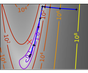

In scipy, you can use the Newton method by setting method to Newton-CG in scipy.optimize.minimize(). Here, CG refers to the fact that an internal inversion of the Hessian is performed by conjugate gradient

>>> deff(x):# The rosenbrock function
... return.5*(1-x[0])**2+(x[1]-x[0]**2)**2
>>> defjacobian(x):
... returnnp.array((-2*.5*(1-x[0])-4*x[0]*(x[1]-x[0]**2),2*(x[1]-x[0]**2)))
>>> optimize.minimize(f,[2,-1],method="Newton-CG",jac=jacobian)
     fun: 1.5...e-15
     jac: array([  1.0575...e-07,  -7.4832...e-08])
 message: ...'Optimization terminated successfully.'
    nfev: 11
    nhev: 0
     nit: 10
    njev: 52
  status: 0
 success: True
       x: array([0.99999...,  0.99999...])

Note that compared to a conjugate gradient (above), Newton’s method has required less function evaluations, but more gradient evaluations, as it uses it to approximate the Hessian. Let’s compute the Hessian and pass it to the algorithm:

>>> defhessian(x):# Computed with sympy
... returnnp.array(((1-4*x[1]+12*x[0]**2,-4*x[0]),(-4*x[0],2)))
>>> optimize.minimize(f,[2,-1],method="Newton-CG",jac=jacobian,hess=hessian)
     fun: 1.6277...e-15
     jac: array([  1.1104...e-07,  -7.7809...e-08])
 message: ...'Optimization terminated successfully.'
    nfev: 11
    nhev: 10
     nit: 10
    njev: 20
  status: 0
 success: True
       x: array([0.99999...,  0.99999...])

Note

At very high-dimension, the inversion of the Hessian can be costly and unstable (large scale > 250).

Note

Newton optimizers should not to be confused with Newton’s root finding method, based on the same principles, scipy.optimize.newton().

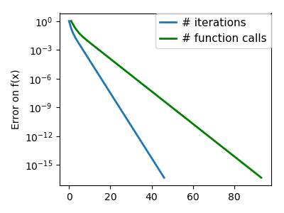
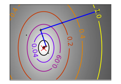
Quasi-Newton methods: approximating the Hessian on the fly¶

BFGS: BFGS (Broyden-Fletcher-Goldfarb-Shanno algorithm) refines at each step an approximation of the Hessian.

2.7.3. Full code examples ¶

2.7.4. Examples for the mathematical optimization chapter ¶

Noisy optimization problem

Smooth vs non-smooth

Curve fitting

Convex function

Finding a minimum in a flat neighborhood

Optimization with constraints

Brent’s method

Constraint optimization: visualizing the geometry

Plotting the comparison of optimizers

Alternating optimization

Gradient descent

Gallery generated by Sphinx-Gallery

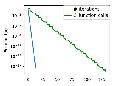
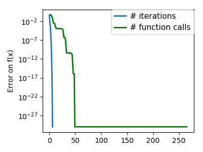
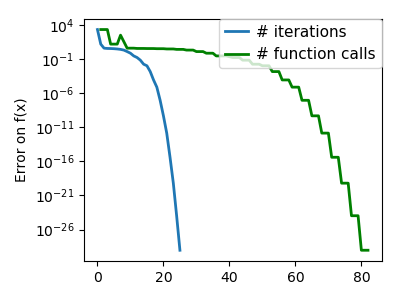
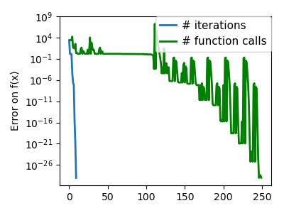
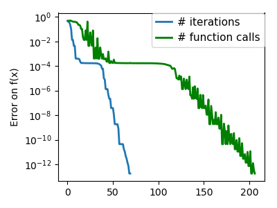
An ill-conditioned quadratic function:

On a exactly quadratic function, BFGS is not as fast as Newton’s method, but still very fast.

An ill-conditioned non-quadratic function:

Here BFGS does better than Newton, as its empirical estimate of the curvature is better than that given by the Hessian.

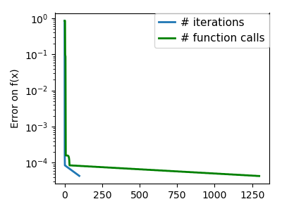
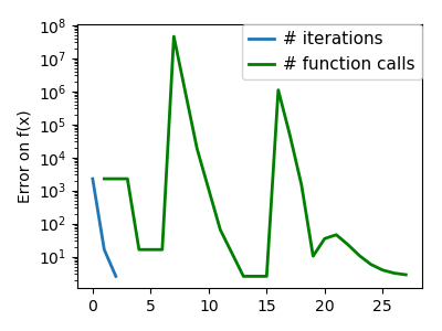
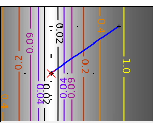
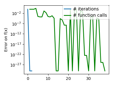
An ill-conditioned very non-quadratic function: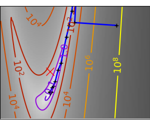

>>> deff(x):# The rosenbrock function
... return.5*(1-x[0])**2+(x[1]-x[0]**2)**2
>>> defjacobian(x):
... returnnp.array((-2*.5*(1-x[0])-4*x[0]*(x[1]-x[0]**2),2*(x[1]-x[0]**2)))
>>> optimize.minimize(f,[2,-1],method="BFGS",jac=jacobian)
      fun: 2.6306...e-16
 hess_inv: array([[0.99986...,  2.0000...],
       [2.0000...,  4.498...]])
      jac: array([  6.7089...e-08,  -3.2222...e-08])
  message: ...'Optimization terminated successfully.'
     nfev: 10
      nit: 8
     njev: 10
   status: 0
  success: True
        x: array([1.        ,  0.99999...])

L-BFGS: Limited-memory BFGS Sits between BFGS and conjugate gradient: in very high dimensions (> 250) the Hessian matrix is too costly to compute and invert. L-BFGS keeps a low-rank version. In addition, box bounds are also supported by L-BFGS-B:

>>> deff(x):# The rosenbrock function
... return.5*(1-x[0])**2+(x[1]-x[0]**2)**2
>>> defjacobian(x):
... returnnp.array((-2*.5*(1-x[0])-4*x[0]*(x[1]-x[0]**2),2*(x[1]-x[0]**2)))
>>> optimize.minimize(f,[2,2],method="L-BFGS-B",jac=jacobian)
      fun: 1.4417...e-15
 hess_inv: <2x2 LbfgsInvHessProduct with dtype=float64>
      jac: array([  1.0233...e-07,  -2.5929...e-08])
  message: ...'CONVERGENCE: NORM_OF_PROJECTED_GRADIENT_<=_PGTOL'
     nfev: 17
      nit: 16
   status: 0
  success: True
        x: array([1.0000...,  1.0000...])

2.7.4.12. Gradient-less methods ¶

A shooting method: the Powell algorithm¶

Almost a gradient approach

An ill-conditioned quadratic function:

Powell’s method isn’t too sensitive to local ill-conditionning in low dimensions

An ill-conditioned very non-quadratic function: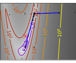

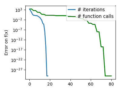
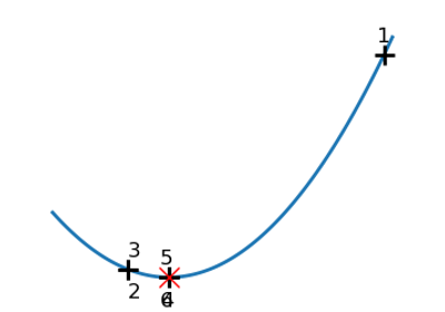
Simplex method: the Nelder-Mead¶

The Nelder-Mead algorithms is a generalization of dichotomy approaches to high-dimensional spaces. The algorithm works by refining a simplex, the generalization of intervals and triangles to high-dimensional spaces, to bracket the minimum.

Strong points: it is robust to noise, as it does not rely on computing gradients. Thus it can work on functions that are not locally smooth such as experimental data points, as long as they display a large-scale bell-shape behavior. However it is slower than gradient-based methods on smooth, non-noisy functions.

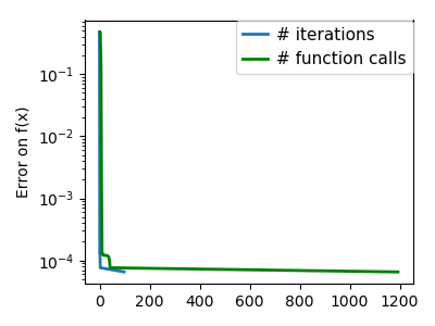
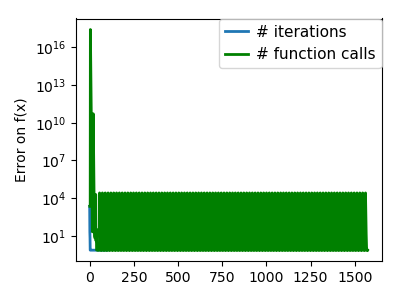
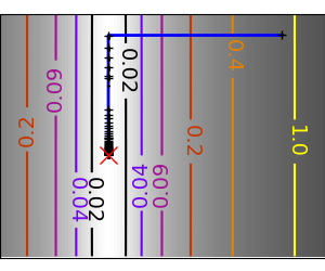
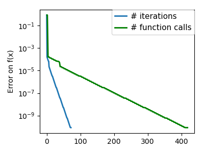
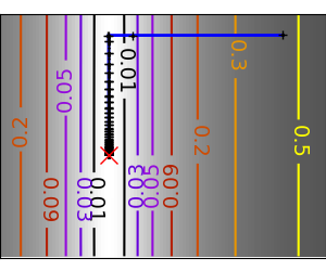
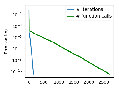
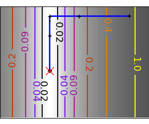
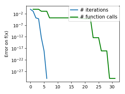
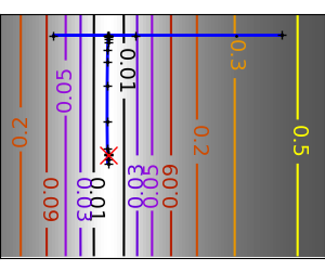
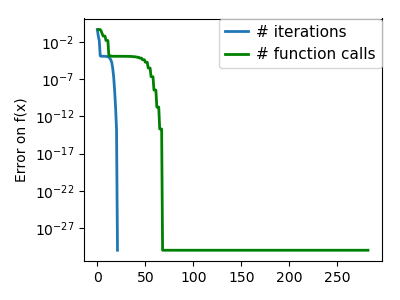
An ill-conditioned non-quadratic function: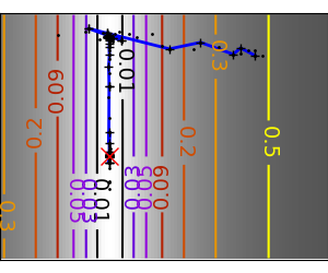
An ill-conditioned very non-quadratic function: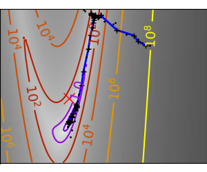

Using the Nelder-Mead solver in scipy.optimize.minimize():

>>> deff(x):# The rosenbrock function
... return.5*(1-x[0])**2+(x[1]-x[0]**2)**2
>>> optimize.minimize(f,[2,-1],method="Nelder-Mead")
 final_simplex: (array([[1.0000...,  1.0000...],
       [0.99998... ,  0.99996... ],
       [1.0000...,  1.0000... ]]), array([1.1152...e-10,   1.5367...e-10,   4.9883...e-10]))
           fun: 1.1152...e-10
       message: ...'Optimization terminated successfully.'
          nfev: 111
           nit: 58
        status: 0
       success: True
             x: array([1.0000...,  1.0000...])

2.7.4.13. Global optimizers ¶

If your problem does not admit a unique local minimum (which can be hard to test unless the function is convex), and you do not have prior information to initialize the optimization close to the solution, you may need a global optimizer.

Brute force: a grid search¶

scipy.optimize.brute() evaluates the function on a given grid of parameters and returns the parameters corresponding to the minimum value. The parameters are specified with ranges given to numpy.mgrid. By default, 20 steps are taken in each direction:

>>> deff(x):# The rosenbrock function
... return.5*(1-x[0])**2+(x[1]-x[0]**2)**2
>>> optimize.brute(f,((-1,2),(-1,2)))
array([1.0000...,  1.0000...])

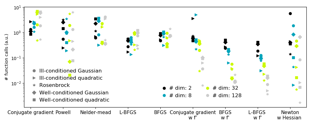
2.7.5. Practical guide to optimization with scipy ¶

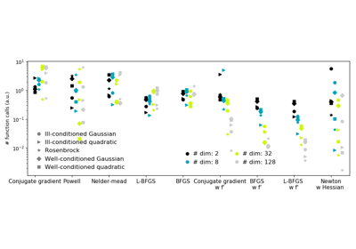
2.7.5.1. Choosing a method ¶

All methods are exposed as the method argument of scipy.optimize.minimize().

../../_images/sphx_glr_plot_compare_optimizers_001.png

Without knowledge of the gradient:
	In general, prefer BFGS or L-BFGS, even if you have to approximate numerically gradients. These are also the default if you omit the parameter `method` - depending if the problem has constraints or bounds On well-conditioned problems, Powell and Nelder-Mead, both gradient-free methods, work well in high dimension, but they collapse for ill-conditioned problems.
With knowledge of the gradient:
	BFGS or L-BFGS. Computational overhead of BFGS is larger than that L-BFGS, itself larger than that of conjugate gradient. On the other side, BFGS usually needs less function evaluations than CG. Thus conjugate gradient method is better than BFGS at optimizing computationally cheap functions.
With the Hessian:
	If you can compute the Hessian, prefer the Newton method (Newton-CG or TCG).
If you have noisy measurements:
	Use Nelder-Mead or Powell.

2.7.5.2. Making your optimizer faster ¶

Choose the right method (see above), do compute analytically the gradient and Hessian, if you can.
Use preconditionning when possible.
Choose your initialization points wisely. For instance, if you are running many similar optimizations, warm-restart one with the results of another.
Relax the tolerance if you don’t need precision using the parameter tol.

2.7.5.3. Computing gradients ¶

Computing gradients, and even more Hessians, is very tedious but worth the effort. Symbolic computation with Sympy may come in handy.

Warning

A very common source of optimization not converging well is human error in the computation of the gradient. You can use scipy.optimize.check_grad() to check that your gradient is correct. It returns the norm of the different between the gradient given, and a gradient computed numerically:

>>> optimize.check_grad(f,jacobian,[2,-1])
2.384185791015625e-07

See also scipy.optimize.approx_fprime() to find your errors.

2.7.5.4. Synthetic exercices ¶

../../_images/sphx_glr_plot_exercise_ill_conditioned_001.png

Exercice: A simple (?) quadratic function

Optimize the following function, using K[0] as a starting point:

np.random.seed(0)
K=np.random.normal(size=(100,100))
deff(x):
returnnp.sum((np.dot(K,x-1))**2)+np.sum(x**2)**2

Time your approach. Find the fastest approach. Why is BFGS not working well?

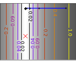
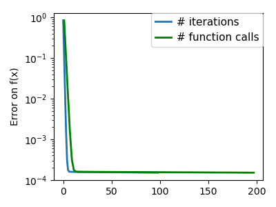
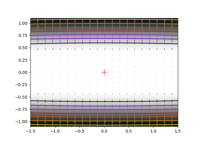
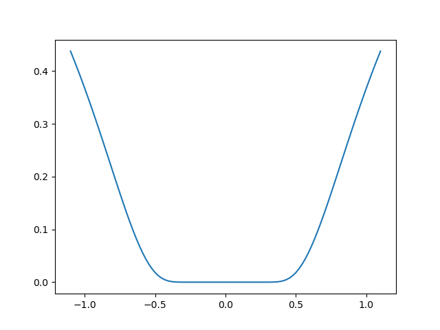
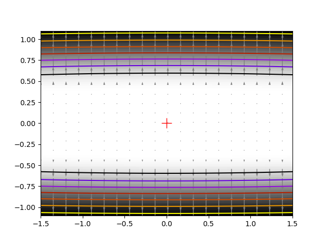
Exercice: A locally flat minimum

Consider the function exp(-1/(.1*x**2 + y**2). This function admits a minimum in (0, 0). Starting from an initialization at (1, 1), try to get within 1e-8 of this minimum point.

2.7.6. Special case: non-linear least-squares ¶

2.7.6.1. Minimizing the norm of a vector function ¶

Least square problems, minimizing the norm of a vector function, have a specific structure that can be used in the Levenberg–Marquardt algorithm implemented in scipy.optimize.leastsq().

Lets try to minimize the norm of the following vectorial function:

>>> deff(x):
... returnnp.arctan(x)-np.arctan(np.linspace(0,1,len(x)))
>>> x0=np.zeros(10)
>>> optimize.leastsq(f,x0)
(array([0.        ,  0.11111111,  0.22222222,  0.33333333,  0.44444444,
        0.55555556,  0.66666667,  0.77777778,  0.88888889,  1.        ]), 2)

This took 67 function evaluations (check it with ‘full_output=1’). What if we compute the norm ourselves and use a good generic optimizer (BFGS):

>>> defg(x):
... returnnp.sum(f(x)**2)
>>> optimize.minimize(g,x0,method="BFGS")
  fun: 2.6940...e-11
 hess_inv: array([[...
 ...
           ...]])
      jac: array([...
 ...
           ...])
  message: ...'Optimization terminated successfully.'
     nfev: 144
      nit: 11
     njev: 12
   status: 0
  success: True
        x: array([-7.3...e-09,   1.1111...e-01,   2.2222...e-01, 3.3333...e-01,
        4.4444...e-01,   5.5555...e-01, 6.6666...e-01,   7.7777...e-01,
        8.8889...e-01, 1.0000...e+00])

BFGS needs more function calls, and gives a less precise result.

Note

leastsq is interesting compared to BFGS only if the dimensionality of the output vector is large, and larger than the number of parameters to optimize.

Warning

If the function is linear, this is a linear-algebra problem, and should be solved with scipy.linalg.lstsq().

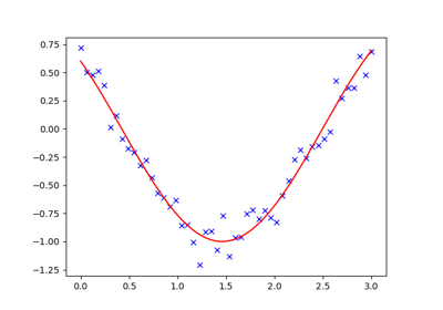
2.7.6.2. Curve fitting ¶

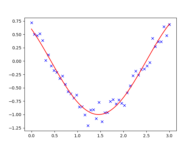
../../_images/sphx_glr_plot_curve_fitting_001.png

Least square problems occur often when fitting a non-linear to data. While it is possible to construct our optimization problem ourselves, scipy provides a helper function for this purpose: scipy.optimize.curve_fit():

>>> deff(t,omega,phi):
... returnnp.cos(omega*t+phi)
>>> x=np.linspace(0,3,50)
>>> y=f(x,1.5,1)+.1*np.random.normal(size=50)
>>> optimize.curve_fit(f,x,y)
(array([1.5185...,  0.92665...]), array([[ 0.00037..., -0.00056...],
       [-0.0005...,  0.00123...]]))

Exercise

Do the same with omega = 3. What is the difficulty?

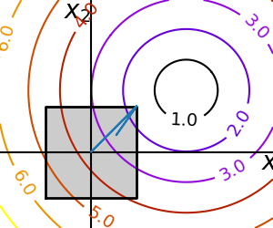
2.7.7. Optimization with constraints ¶

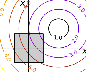
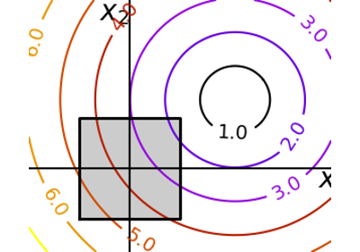
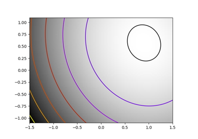
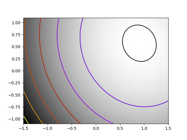
2.7.7.1. Box bounds ¶

Box bounds correspond to limiting each of the individual parameters of the optimization. Note that some problems that are not originally written as box bounds can be rewritten as such via change of variables. Both scipy.optimize.minimize_scalar() and scipy.optimize.minimize() support bound constraints with the parameter bounds:

>>> deff(x):
... returnnp.sqrt((x[0]-3)**2+(x[1]-2)**2)
>>> optimize.minimize(f,np.array([0,0]),bounds=((-1.5,1.5),(-1.5,1.5)))
      fun: 1.5811...
 hess_inv: <2x2 LbfgsInvHessProduct with dtype=float64>
      jac: array([-0.94868..., -0.31622...])
  message: ...'CONVERGENCE: NORM_OF_PROJECTED_GRADIENT_<=_PGTOL'
     nfev: 9
      nit: 2
   status: 0
  success: True
        x: array([1.5,  1.5])

../../_images/sphx_glr_plot_constraints_002.png

2.7.7.2. General constraints ¶

Equality and inequality constraints specified as functions: $f(x) = 0$ and $g(x) < 0$ .

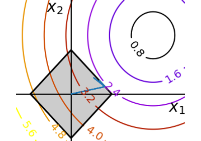
scipy.optimize.fmin_slsqp() Sequential least square programming: equality and inequality constraints: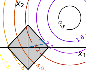

../../_images/sphx_glr_plot_non_bounds_constraints_001.png

>>> deff(x):
... returnnp.sqrt((x[0]-3)**2+(x[1]-2)**2)
>>> defconstraint(x):
... returnnp.atleast_1d(1.5-np.sum(np.abs(x)))
>>> x0=np.array([0,0])
>>> optimize.minimize(f,x0,constraints={"fun":constraint,"type":"ineq"})
     fun: 2.4748...
     jac: array([-0.70708..., -0.70712...])
 message: ...'Optimization terminated successfully.'
    nfev: 20
     nit: 5
    njev: 5
  status: 0
 success: True
       x: array([1.2500...,  0.2499...])

Warning

The above problem is known as the Lasso problem in statistics, and there exist very efficient solvers for it (for instance in scikit-learn). In general do not use generic solvers when specific ones exist.

Lagrange multipliers

If you are ready to do a bit of math, many constrained optimization problems can be converted to non-constrained optimization problems using a mathematical trick known as Lagrange multipliers.

2.7.8. Full code examples ¶

2.7.9. Examples for the mathematical optimization chapter ¶

Noisy optimization problem

Smooth vs non-smooth

Curve fitting

Convex function

Finding a minimum in a flat neighborhood

Optimization with constraints

Brent’s method

Constraint optimization: visualizing the geometry

Plotting the comparison of optimizers

Alternating optimization

Gradient descent

Gallery generated by Sphinx-Gallery

2.7. Mathematical optimization: finding minima of functions¶

2.7.1. Knowing your problem ¶

2.7.1.1. Convex versus non-convex optimization ¶

2.7.1.2. Smooth and non-smooth problems ¶

2.7.1.3. Noisy versus exact cost functions ¶

2.7.1.4. Constraints ¶

2.7.2. A review of the different optimizers ¶

2.7.2.1. Getting started: 1D optimization ¶

2.7.2.2. Gradient based methods ¶

Some intuitions about gradient descent¶

Conjugate gradient descent¶

2.7.2.3. Newton and quasi-newton methods ¶

Newton methods: using the Hessian (2nd differential)¶

Quasi-Newton methods: approximating the Hessian on the fly¶

2.7.3. Full code examples ¶

2.7.4. Examples for the mathematical optimization chapter ¶

2.7.4.12. Gradient-less methods ¶

A shooting method: the Powell algorithm¶

Simplex method: the Nelder-Mead¶

2.7.4.13. Global optimizers ¶

Brute force: a grid search¶

2.7.5. Practical guide to optimization with scipy ¶

2.7.5.1. Choosing a method ¶

2.7.5.2. Making your optimizer faster ¶

2.7.5.3. Computing gradients ¶

2.7.5.4. Synthetic exercices ¶

2.7.6. Special case: non-linear least-squares ¶

2.7.6.1. Minimizing the norm of a vector function ¶

2.7.6.2. Curve fitting ¶

2.7.7. Optimization with constraints ¶

2.7.7.1. Box bounds ¶

2.7.7.2. General constraints ¶

2.7.8. Full code examples ¶

2.7.9. Examples for the mathematical optimization chapter ¶

Table Of Contents

Previous topic

Next topic

This Page